
-


人工智能
站-
热门城市 全国站>
-
其他省市
-
-

 15692118659
 小职
2021-09-01
来源 :CSDN「小陈phd」
阅读 2838
评论 0
小职
2021-09-01
来源 :CSDN「小陈phd」
阅读 2838
评论 0
摘要:本文主要介绍了人工智能深度学习之目标检测——RCNN,通过具体的内容向大家展现,希望对大家人工智能深度学习的学习有所帮助。
本文主要介绍了人工智能深度学习之目标检测——RCNN,通过具体的内容向大家展现,希望对大家人工智能深度学习的学习有所帮助。

Selective Search
背景:事先不知道需要检测哪个类别,且候选目标存在层级关系与尺度关系
常规解决方法:穷举法·,在原始图片上进行不同尺度不同大小的滑窗,获取每个可能的位置
弊端:计算量大,且尺度不能兼顾
Selective Search:通过视觉特征减少分类可能性
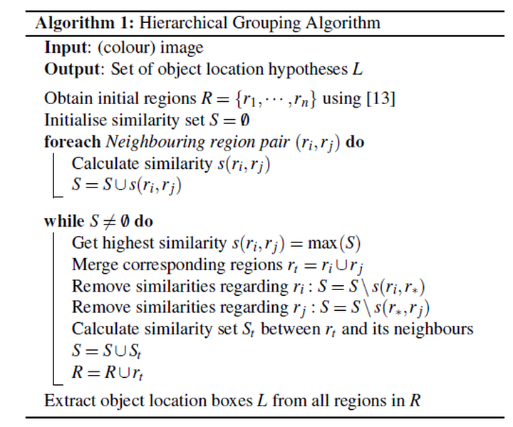
算法步骤
基于图的图像分割方法初始化区域(图像分割为很多很多小块)
循环
使用贪心策略计算相邻区域相似度,每次合并相似的两块
直到剩下一块
结束
如何保证特征多样性
颜色空间变换,RGB,i,Lab,HSV,
距离计算方式
颜色距离
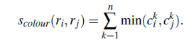
计算每个通道直方图
取每个对应bins的直方图最小值
直方图大小加权区域/总区域
纹理距离
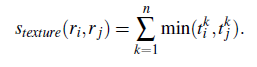
计算每个区域的快速sift特征(方向个数为8)
每个通道bins为2
其他用颜色距离
优先合并小区域
单纯通过颜色和纹理合并
合并区域会不断吞并,造成多尺度应用在局部问题上,无法全局多尺度
解决方法:给小区域更多权重
.区域的合适度度距离
除了考虑每个区域特征的吻合程度,还要考虑区域吻合度(合并后的区域尽量规范,不能出现断崖式的区域)
直接需求就是区域的外接矩形的重合面积要大
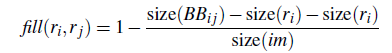
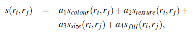
加权综合衡量距离
给予各种距离整合一些区域建议,加权综合考虑
参数初始化多样性
通过多种参数初始化图像分割
区域打分
代码实现
# -*- coding: utf-8 -*-
from __future__ import division
import cv2 as cv
import skimage.io
import skimage.feature
import skimage.color
import skimage.transform
import skimage.util
import skimage.segmentation
import numpy
# "Selective Search for Object Recognition" by J.R.R. Uijlings et al.
#
# - Modified version with LBP extractor for texture vectorization
def _generate_segments(im_orig, scale, sigma, min_size):
"""
segment smallest regions by the algorithm of Felzenswalb and
Huttenlocher
"""
# open the Image
im_mask = skimage.segmentation.felzenszwalb(
skimage.util.img_as_float(im_orig), scale=scale, sigma=sigma,
min_size=min_size)
# merge mask channel to the image as a 4th channel
im_orig = numpy.append(
im_orig, numpy.zeros(im_orig.shape[:2])[:, :, numpy.newaxis], axis=2)
im_orig[:, :, 3] = im_mask
return im_orig
def _sim_colour(r1, r2):
"""
calculate the sum of histogram intersection of colour
"""
return sum([min(a, b) for a, b in zip(r1["hist_c"], r2["hist_c"])])
def _sim_texture(r1, r2):
"""
calculate the sum of histogram intersection of texture
"""
return sum([min(a, b) for a, b in zip(r1["hist_t"], r2["hist_t"])])
def _sim_size(r1, r2, imsize):
"""
calculate the size similarity over the image
"""
return 1.0 - (r1["size"] + r2["size"]) / imsize
def _sim_fill(r1, r2, imsize):
"""
calculate the fill similarity over the image
"""
bbsize = (
(max(r1["max_x"], r2["max_x"]) - min(r1["min_x"], r2["min_x"]))
* (max(r1["max_y"], r2["max_y"]) - min(r1["min_y"], r2["min_y"]))
)
return 1.0 - (bbsize - r1["size"] - r2["size"]) / imsize
def _calc_sim(r1, r2, imsize):
return (_sim_colour(r1, r2) + _sim_texture(r1, r2)
+ _sim_size(r1, r2, imsize) + _sim_fill(r1, r2, imsize))
def _calc_colour_hist(img):
"""
calculate colour histogram for each region
the size of output histogram will be BINS * COLOUR_CHANNELS(3)
number of bins is 25 as same as [uijlings_ijcv2013_draft.pdf]
extract HSV
"""
BINS = 25
hist = numpy.array([])
for colour_channel in (0, 1, 2):
# extracting one colour channel
c = img[:, colour_channel]
# calculate histogram for each colour and join to the result
hist = numpy.concatenate(
[hist] + [numpy.histogram(c, BINS, (0.0, 255.0))[0]])
# L1 normalize
hist = hist / len(img)
return hist
def _calc_texture_gradient(img):
"""
calculate texture gradient for entire image
The original SelectiveSearch algorithm proposed Gaussian derivative
for 8 orientations, but we use LBP instead.
output will be [height(*)][width(*)]
"""
ret = numpy.zeros((img.shape[0], img.shape[1], img.shape[2]))
for colour_channel in (0, 1, 2):
ret[:, :, colour_channel] = skimage.feature.local_binary_pattern(
img[:, :, colour_channel], 8, 1.0)
# LBP特征
return ret
def _calc_texture_hist(img):
"""
calculate texture histogram for each region
calculate the histogram of gradient for each colours
the size of output histogram will be
BINS * ORIENTATIONS * COLOUR_CHANNELS(3)
"""
BINS = 10
hist = numpy.array([])
for colour_channel in (0, 1, 2):
# mask by the colour channel
fd = img[:, colour_channel]
# calculate histogram for each orientation and concatenate them all
# and join to the result
hist = numpy.concatenate(
[hist] + [numpy.histogram(fd, BINS, (0.0, 1.0))[0]])
# L1 Normalize
hist = hist / len(img)
return hist
def _extract_regions(img):
R = {}
# get hsv image
hsv = skimage.color.rgb2hsv(img[:, :, :3])
# pass 1: count pixel positions
for y, i in enumerate(img):
for x, (r, g, b, l) in enumerate(i):
# initialize a new region
if l not in R:
R[l] = {
"min_x": 0xffff, "min_y": 0xffff,
"max_x": 0, "max_y": 0, "labels": [l]}
# bounding box
if R[l]["min_x"] > x:
R[l]["min_x"] = x
if R[l]["min_y"] > y:
R[l]["min_y"] = y
if R[l]["max_x"] < x:
R[l]["max_x"] = x
if R[l]["max_y"] < y:
R[l]["max_y"] = y
# pass 2: calculate texture gradient
tex_grad = _calc_texture_gradient(img)
# pass 3: calculate colour histogram of each region
for k, v in list(R.items()):
# colour histogram
masked_pixels = hsv[:, :, :][img[:, :, 3] == k]
R[k]["size"] = len(masked_pixels / 4)
R[k]["hist_c"] = _calc_colour_hist(masked_pixels)
# texture histogram
R[k]["hist_t"] = _calc_texture_hist(tex_grad[:, :][img[:, :, 3] == k])
return R
def _extract_neighbours(regions):
def intersect(a, b):
if (a["min_x"] < b["min_x"] < a["max_x"]
and a["min_y"] < b["min_y"] < a["max_y"]) or (
a["min_x"] < b["max_x"] < a["max_x"]
and a["min_y"] < b["max_y"] < a["max_y"]) or (
a["min_x"] < b["min_x"] < a["max_x"]
and a["min_y"] < b["max_y"] < a["max_y"]) or (
a["min_x"] < b["max_x"] < a["max_x"]
and a["min_y"] < b["min_y"] < a["max_y"]):
return True
return False
R = list(regions.items())
neighbours = []
for cur, a in enumerate(R[:-1]):
for b in R[cur + 1:]:
if intersect(a[1], b[1]):
neighbours.append((a, b))
return neighbours
def _merge_regions(r1, r2):
new_size = r1["size"] + r2["size"]
rt = {
"min_x": min(r1["min_x"], r2["min_x"]),
"min_y": min(r1["min_y"], r2["min_y"]),
"max_x": max(r1["max_x"], r2["max_x"]),
"max_y": max(r1["max_y"], r2["max_y"]),
"size": new_size,
"hist_c": (
r1["hist_c"] * r1["size"] + r2["hist_c"] * r2["size"]) / new_size,
"hist_t": (
r1["hist_t"] * r1["size"] + r2["hist_t"] * r2["size"]) / new_size,
"labels": r1["labels"] + r2["labels"]
}
return rt
def selective_search(im_orig, scale=1.0, sigma=0.8, min_size=50):
'''Selective Search
Parameters
----------
im_orig : ndarray
Input image
scale : int
Free parameter. Higher means larger clusters in felzenszwalb segmentation.
sigma : float
Width of Gaussian kernel for felzenszwalb segmentation.
min_size : int
Minimum component size for felzenszwalb segmentation.
Returns
-------
img : ndarray
image with region label
region label is stored in the 4th value of each pixel [r,g,b,(region)]
regions : array of dict
[
{
'rect': (left, top, width, height),
'labels': [...],
'size': component_size
},
...
]
'''
# 期待输入3通道图片
assert im_orig.shape[2] == 3, "3ch image is expected"
# load image and get smallest regions
# region label is stored in the 4th value of each pixel [r,g,b,(region)]
# 基于图方法生成图的最小区域,
img = _generate_segments(im_orig, scale, sigma, min_size)
# (512, 512, 4)
# print(img.shape)
# cv2.imshow("res1", im_orig)
# print(type(img))
# # img = cv2.cvtColor(img,cv2.COLOR_RGB2BGR)
# cv2.imshow("res",img)
# cv2.waitKey(0)
# # print(img)
# exit()
if img is None:
return None, {}
imsize = img.shape[0] * img.shape[1]
# 拓展区域
R = _extract_regions(img)
# extract neighbouring information
neighbours = _extract_neighbours(R)
# calculate initial similarities
S = {}
for (ai, ar), (bi, br) in neighbours:
S[(ai, bi)] = _calc_sim(ar, br, imsize)
# hierarchal search
while S != {}:
# get highest similarity
i, j = sorted(S.items(), key=lambda i: i[1])[-1][0]
# merge corresponding regions
t = max(R.keys()) + 1.0
R[t] = _merge_regions(R[i], R[j])
# mark similarities for regions to be removed
key_to_delete = []
for k, v in list(S.items()):
if (i in k) or (j in k):
key_to_delete.append(k)
# remove old similarities of related regions
for k in key_to_delete:
del S[k]
# calculate similarity set with the new region
for k in [a for a in key_to_delete if a != (i, j)]:
n = k[1] if k[0] in (i, j) else k[0]
S[(t, n)] = _calc_sim(R[t], R[n], imsize)
regions = []
for k, r in list(R.items()):
regions.append({
'rect': (
r['min_x'], r['min_y'],
r['max_x'] - r['min_x'], r['max_y'] - r['min_y']),
'size': r['size'],
'labels': r['labels']
})
return img, regions
测试
# -*- coding: utf-8 -*-
from __future__ import (
division,
print_function,
)
import cv2 as cv
import skimage.data
import matplotlib.pyplot as plt
import matplotlib.patches as mpatches
import selectivesearch
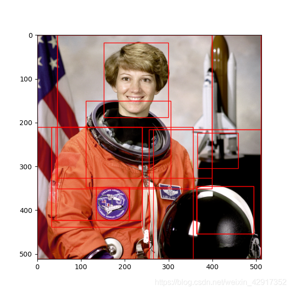
def main():
# loading astronaut image
img = skimage.data.astronaut()
# print(type(img))
# img = cv.cvtColor(img,cv.COLOR_RGB2BGR)
# cv.imshow("res",img)
# cv.waitKey(0)
# # print(img)
# exit()
# perform selective search
img_lbl, regions = selectivesearch.selective_search(
img, scale=500, sigma=0.9, min_size=10)
candidates = set()
for r in regions:
# excluding same rectangle (with different segments)
if r['rect'] in candidates:
continue
# excluding regions smaller than 2000 pixels
if r['size'] < 2000:
continue
# distorted rects
x, y, w, h = r['rect']
if w / h > 1.2 or h / w > 1.2:
continue
candidates.add(r['rect'])
# draw rectangles on the original image
fig, ax = plt.subplots(ncols=1, nrows=1, figsize=(6, 6))
ax.imshow(img)
for x, y, w, h in candidates:
print(x, y, w, h)
rect = mpatches.Rectangle(
(x, y), w, h, fill=False, edgecolor='red', linewidth=1)
ax.add_patch(rect)
plt.show()
if __name__ == "__main__":
main()
测试结果
RCNN
算法步骤
产生目标区域候选
CNN目标特征提取
使用的AlexNet
imageNet预训练迁移学习,只训练全连接层
采用的全连接层输出(导致输入大小必须固定)
目标种类分类器
SVM困难样本挖掘方法,正样本—>正样本 ,iou>0.3 == 负样本
贪婪非极大值抑制 NMS
根据分类器的类别分类概率做排序,假设从小到大属于正样本的概率 分别为A、B、C、D、E、F。
从最大概率矩形框F开始,分别判断A~E与F的重叠度IOU是否大于某个设定的阈值
假设B、D与F的重叠度超过阈值,那么就扔掉B、D;并标记第一个矩形框F,是我们保留下来的。
从剩下的矩形框A、C、E中,选择概率最大的E,然后判断E与A、C的重叠度,重叠度大于一定的阈值,那么就扔掉;并标记E是我们保留下来的第二个矩形框。
就这样一直重复,找到所有被保留下来的矩形框。
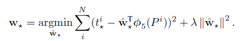
BoundingBox回归
微调回归框
一个区域位置
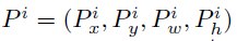
位置映射真实位置
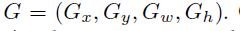
转换偏移量参数

映射关系式
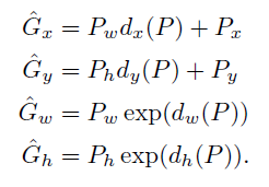
选用pool5层
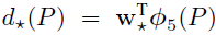
最小化w
不使用全连接的输出作为非极大抑制的输入,而是训练很多的SVM。
因为CNN需要大量的样本,当正样本设置为真实BoundingBox时效果很差,而IOU>0.5相当于30倍的扩充了样本数量。而我们近将CNN结果作为一个初选,然后用困难负样本挖掘的SVM作为第二次筛选就好多了
缺点:时间代价太高了
我是小职,记得找我
✅ 解锁高薪工作
✅ 免费获取基础课程·答疑解惑·职业测评

 喜欢 | 0
 不喜欢 | 0


您输入的评论内容中包含违禁敏感词
我知道了

请输入正确的手机号码
请输入正确的验证码
您今天的短信下发次数太多了,明天再试试吧!
我们会在第一时间安排职业规划师联系您!
您也可以联系我们的职业规划师咨询:

版权所有 职坐标-IT技术咨询与就业发展一体化服务 沪ICP备13042190号-4
上海海同信息科技有限公司 Copyright ©2015 www.zhizuobiao.com,All Rights Reserved.
 沪公网安备 31011502005948号


 索取资料
索取资料

 答疑解惑
答疑解惑

 技术交流
技术交流

 职业测评
职业测评

 面试技巧
面试技巧

 高薪秘笈
高薪秘笈